TSegFormer: 3D Tooth Segmentation in Intraoral Scans with Geometry Guided Transformer
代码复现比较困难的地方是数据集的处理,因此下面主要介绍数据集处理的部分
个人使用的数据集
数据集需要有:三维点坐标以及点对应的标签
数据集处理
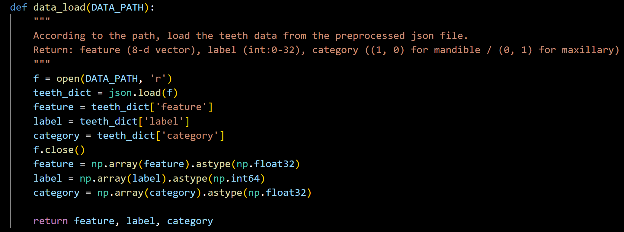
首先根据 data.py 和论文,我们可以得出数据集的格式:
feature,8 维向量,分别是 3 维点坐标+3 维法向量+高斯曲率+点”曲率”
label,标签,0-32,0 是牙龈
category,(1,0)为下颌骨,(0,1)为上颌骨
具体实现如下:
1.从.obj 文件中提取出点坐标
def read_obj_vertices(file_path):
    vertices = []
    with open(file_path, 'r') as file:
        for line in file:
            if line.startswith('v '):  # 仅处理顶点行
                parts = line.strip().split()
                x, y, z = map(float, parts[1:4])  # 提取 x,y,z 坐标
                vertices.append([x,  y, z])
    return np.array(vertices)
2.计算法线,这里通过 open3d 计算
pcd = o3d.geometry.PointCloud()
pcd.points  = o3d.utility.Vector3dVector(vertex_array)
pcd.estimate_normals( search_param=o3d.geometry.KDTreeSearchParamHybrid(radius=5.5,  max_nn=30))
normals_array = np.asarray(pcd.normals)
3.计算高斯曲率
Deepseek 生成的(不保证正确性),最后数据很大,所以在最后处理时,所有的数据进行了归一化处理
def compute_gaussian_curvature(points, normals, radius=0.1):
    """
    计算点云中每个点的高斯曲率

    参数:
        points: numpy 数组,形状为(N, 3),表示点云中的点
        normals: numpy 数组,形状为(N, 3),表示每个点的法向量
        radius: 浮点数,用于确定邻域范围的半径

    返回:
        gaussian_curvatures: numpy 数组,形状为(N,),每个点的高斯曲率
    """
    # 构建 KD 树以快速查找邻域点
    tree = KDTree(points)

    gaussian_curvatures = np.zeros(points.shape[0])

    for i in range(points.shape[0]):
        # 找到以当前点为中心,半径为 radius 的邻域内的点的索引
        indices = tree.query_ball_point(points[i], radius)
        neighborhood_points = points[indices]

        # 如果邻域内点数不足,跳过
        if len(neighborhood_points) < 3:
            gaussian_curvatures[i] = 0
            continue

        # 计算协方差矩阵
        mean_point = np.mean(neighborhood_points, axis=0)
        centered_points = neighborhood_points - mean_point
        cov_matrix = np.dot(centered_points.T, centered_points)

        # 计算协方差矩阵的特征值
        eigenvalues, _ = np.linalg.eig(cov_matrix)
        eigenvalues = np.sort(eigenvalues)[::-1]

        # 计算主曲率(这里简化处理,实际可能需要更复杂的曲面拟合)
        k1 = eigenvalues[0]
        k2 = eigenvalues[1]

        # 高斯曲率是主曲率的乘积
        gaussian_curvatures[i] = k1 * k2

    return gaussian_curvatures
4.计算点“曲率”
Deepseek 生成的(不保证正确性)
def compute_point_curvature_new(points, normals, radius=0.1):
    """
    计算点云中每个点的新定义的点“曲率”

    参数:
    points (numpy.ndarray):  点云数据,形状为 (n_points, 3),其中 n_points 是点的数量
    normals (numpy.ndarray):  点云的法向量,形状为 (n_points, 3)
    radius (float): 邻域半径,默认为 0.1

    返回:
    numpy.ndarray:  每个点的曲率,形状为 (n_points,)
    """
    n_points = points.shape[0]
    curvatures = np.zeros(n_points)

    # 使用 sklearn 的 NearestNeighbors 来查找每个点的邻域
    nbrs = NearestNeighbors(radius=radius, algorithm='ball_tree').fit(points)

    for i in range(n_points):
        # 查找当前点的邻域点
        distances, indices = nbrs.radius_neighbors([points[i]],  return_distance=True)
        neighbor_indices = indices[0]

        if len(neighbor_indices) > 1:
            # 获取当前点的法向量
            current_normal = normals[i]

            # 获取邻域点的法向量
            neighbor_normals = normals[neighbor_indices]

            # 计算当前点法向量与邻域点法向量的夹角余弦值
            cos_angles = np.dot(neighbor_normals,  current_normal)

            # 计算曲率,这里定义为夹角余弦值的平均值
            curvature = np.mean(cos_angles)
            curvatures[i] = curvature

    return curvatures
5.最终得到的数据进行归一化处理
def pc_normalize(pc):
    centroid = np.mean(pc, axis=0)
    pc = pc - centroid
    m = np.max(np.sqrt(np.sum(pc ** 2, axis=1)))
    pc = pc / m
    return pc

vertices = pc_normalize(vertices)
normals = pc_normalize(normals)
gaussian_curvatures = gaussian_curvatures / 10000000000
6.labels 转换
def number_covert(original):
    num_map = {
        31:1,
        32:2,
        33:3,
        34:4,
        35:5,
        36:6,
        37:7,
        38:8,
        41:9,
        42:10,
        43:11,
        44:12,
        45:13,
        46:14,
        47:15,
        48:16,
        11:17,
        12:18,
        13:19,
        14:20,
        15:21,
        16:22,
        17:23,
        18:24,
        21:25,
        22:26,
        23:27,
        24:28,
        25:29,
        26:30,
        27:31,
        28:32
    }
    new_list = [num_map.get(x,  x) for x in original]
    return new_list
7.修改 data.py
def data_load(DATA_PATH):
    """
    According to the path, load the teeth data from the preprocessed json file.
    Return: feature (8-d vector), label (int:0-32), category ((1, 0) for mandible / (0, 1) for maxillary)
    """
    f = open(DATA_PATH + ".json", 'r')
    teeth_dict = json.load(f)
    label = teeth_dict['labels']
    f.close()

    label = number_covert(label)
    label = np.array(label).astype(np.int64)
    # print(label)
    cat = teeth_dict['jaw']
    if cat == 'lower':
        category = (1, 0)
    else:
        category = (0, 1)
    category = np.array(category).astype(np.float32)
    # print(category)

        feature = np.concatenate((vertices, normals), axis=1)
        feature  = np.concatenate((feature, gaussian_array), axis=1)
        feature  = np.concatenate((feature, curvature_array), axis=1)

    # print(feature)
    return feature, label, category
8.进行训练
python main.py --epochs 200 --num_points 10000